Creating heatmaps of player movements in midcore projects: a short guide
I’ve discussed the importance of heatmaps in midcore projects and their applications in my previous article. Today, I’ll delve into the technical aspects — how we collect user coordinates and display them on a screenshot.
Let’s walk through the process step by step; there are five key stages.
Step one: Transmit player coordinates
First, we transmit the player’s coordinates with each in-game event, such as death, reaching a checkpoint, or achieving a kill with a specific weapon type. To capture a more nuanced view of player movements, we also record their locations at set intervals.
Deciding on the frequency of these logs is a judgment call, influenced heavily by the eventual database size. After extensive testing, we found that transmitting data every 5-7 seconds struck the best balance.
Here’s an example of a log event in JSON format:
{”map”:”MapTutorial”,”frame_rate”:”35”,”x”:”633”,”y”:”-56390”,”graphic settings”:”normal”}
Named scene_performance, this event is sent every five seconds during active sessions. Along with the coordinates, it includes technical details like frame rate and graphics settings.
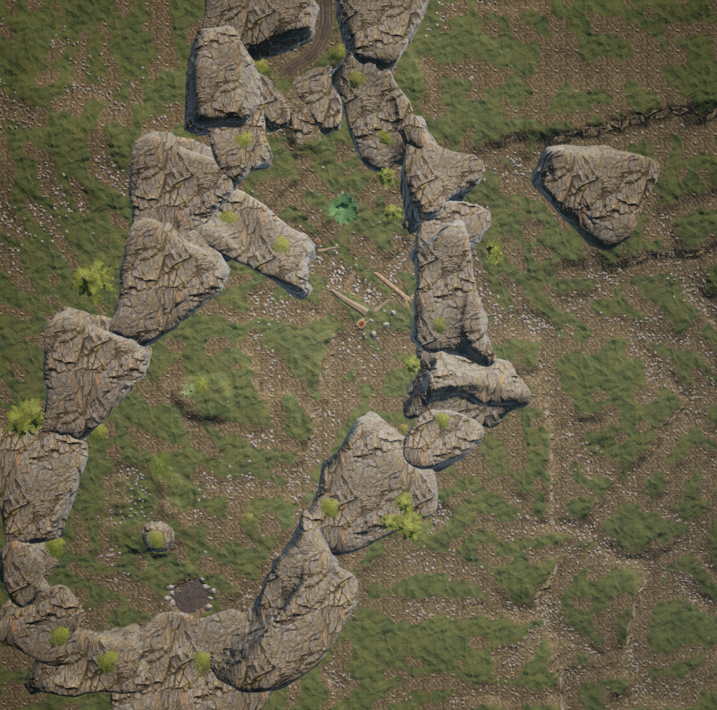
Step two: Capture a screenshot
Next, we take a screenshot of the game level, courtesy of the client developers. For instance, in our midcore off-road driving simulator:
Step three: Align coordinates with the screenshot
With all the necessary data gathered, we can proceed to analyze player movements.
First, we need to align the scale of the player’s coordinates with the screenshot’s dimensions and orientation. In terms of linear algebra, this means projecting each vector from the player’s coordinate space onto our map image’s coordinate space.
To accomplish this in a two-dimensional Cartesian Euclidean space, we employ geometric transformations and transformation matrices, dealing with rotations, scalings, and translations.
Here’s how these transformations might look in Python:
def Normalize(x, y, img_size):
x_out, y_out = x.copy(), y.copy()
shape_x, shape_y = img_size
shift_x = (x_out.min() + x_out.max(right_q))/2
shift_y = (y_out.quantile() + y_out.max())/2
scale_x = abs(1 / (x_out.max() – x_out.min()))*shape_x
scale_y = abs(1 / (y_out.max() – y_out.min()))*shape_y
x_out = (x_out – shift_x)*scale_x
y_out = (y_out – shift_y)*scale_y
return x_out, y_out
def Translate(x, y, shift=None, scale=None, turn=None):
x_out = x.copy()
y_out = y.copy()
if turn is not None:
x_out = x * np.cos(turn) – y * np.sin(turn)
y_out = x * np.sin(turn) + y * np.cos(turn)
if scale is not None:
x_out = x_out * scale[0]
y_out = y_out * scale[1]
if shift is not None:
x_out = x_out + shift[0]
y_out = y_out + shift[1]
return x_out, y_out
In the Normalize function, we transform the cloud of player movement coordinate points, adjusting their size to match that of the screenshot and centering them relative to one another. On the other hand, the Translate function further refines the player’s coordinates by rotating, scaling, and shifting them as needed.
The Normalize function streamlines the alignment process, especially when we are certain that players were on the edges of the map. This certainty allows us to accurately establish the real ranges within the coordinate field where players can be located. Often, we validate this by manually navigating the game to cover the entire map perimeter, ensuring all possible player locations are accounted for. However, this approach has its caveats, particularly when dealing with asymmetrical map shapes. In scenarios where players are unable to cover the entire rectangular area captured in the screenshot, the Normalize function may result in skewed transformations. To mitigate this, we initially apply the Normalize function to the coordinates and subsequently refine the results using the Translate function.
Yet, despite these precautions, there’s still a possibility of encountering “outliers” – data points that lie outside the map’s boundaries in the final image. While these events are relatively rare, it is crucial to identify and remove these anomalies from our analysis to maintain accuracy. Ideally, we aim to filter out the most significant outliers prior to applying the functions described above.
Step four: Overlay coordinates onto the map
Now, we overlay the player coordinates onto the map screenshot. For this, we use the cv2 library in Python, a widely used tool for image processing.
Firstly, initiate an auxiliary matrix that aligns with the original image, ensuring its dimensions are consistent with the scales of our coordinate system. Populate this matrix based on the frequency of player appearances at specific coordinate points.
Here’s a code snippet demonstrating this matrix initialization:
hit_mtx = numpy.zeros((number_y_cells, number_x_cells))
for indX, indY in zip(x, y):
i = int(indX)
j = int(indY)
hit_mtx[j, i] += 1
After creating the matrix, convert it to the appropriate format and size to match our image using the cv2.resize function.
Next, transform the frequency values in the matrix into a matrix of color intensities, representing player densities at specific locations (cells). The higher the frequency value, the more saturated the color, indicating a higher concentration of player activity.
Keep in mind, images are three-dimensional arrays, with the third dimension representing color channels. Therefore, replicate the matrix across each channel to facilitate overlaying the heatmap onto the image.
Here’s how you can construct the color intensity matrix in Python:
def _MaskOfHitArea(img_shape, hit_area, alpha):
mask = np.zeros(img_shape)
mask[:,:,0] = alpha * numpy.float32(hit_area)
mask[:,:,1] = mask[:,:,0].copy()
mask[:,:,2] = mask[:,:,0].copy()
return mask
In this function, alpha < 1 controls the transparency of the overlaid heatmap.
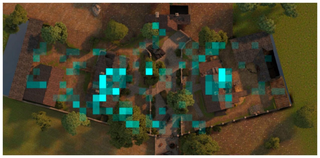
Finally, combine the original image (img) and the color intensity matrix (color_mtx * mask) to produce the heatmap. Use the following formula for the combination:
img * (1 – mask) + mask * color_mtx
Here, color_mtx sets the fill color for the player coordinates.
If there were any issues with the transformations in Step Three, they will become apparent in the heatmap, necessitating a revisit and potential adjustments to Steps Three and Four.
This algorithm can be adapted for different types of events, each distinguished by unique colors. For instance, we used this method to identify and visualize kill locations for different weapon classes in our game (read this article to learn more).
Sniper rifle kill map:
Step five: Make it pretty
Finally, we can enhance our heatmap visualization using the cv2.VideoWriter function, creating dynamic videos of player movements across the map.
This involves iteratively processing specified time intervals, applying the algorithm from Step Four (though not from the entire observation period) to each segment. The number of iterations corresponds to the video’s frame rate.